DRAM and NAND: two technologies, different cycles

Start with what must survive power loss

DRAM and NAND are both semiconductor memories, but they solve different jobs. DRAM stores the active state close to a processor or accelerator and loses data when power disappears; it must be refreshed. NAND flash retains data without power and is organized into pages and erase blocks, so it is suited to SSDs and persistent capacity. AI systems normally need both: weights and active tensors occupy DRAM/HBM while executing; checkpoints, datasets, indexes, and logs live in SSD or networked storage.

1. 1dataset/checkpoint
2. 2NAND SSD
3. 3host DRAM
4. 4HBM
5. 5execution

1. 1persistent capacity staging active state working set

1. 1erase/program constraints
2. 2I/O schedule
3. 3bandwidth
4. 4arithmetic

The distinction changes diagnostics. If a model step stalls while reading shards, storage throughput, queue depth, CPU decompression, or network placement may be limiting. If it stalls inside a kernel, local HBM traffic or compute may matter. Replacing SSDs does not cure a saturated HBM path; adding HBM does not make an unread dataset appear. NVIDIA’s H200 announcement describes a product with 141 GB HBM3e and 4.8 TB/s, while Micron’s HBM3E page describes a memory component. Those sources establish their publishers’ specifications, not an SSD comparison.

Different physical constraints create different economics

DRAM cells trade density for fast, byte-addressable working memory; refresh consumes power and timing margins constrain access. NAND stores charge in cells and normally programs and reads in pages but erases in larger blocks. Updates therefore use an out-of-place process: write fresh data elsewhere, mark old pages invalid, then garbage-collect blocks. Wear leveling spreads program/erase stress, and over-provisioning leaves spare capacity for performance and endurance. A full or write-heavy SSD can behave differently from a fresh, read-mostly drive even at the same interface generation.

A toy example clarifies the non-substitution. Imagine a 1-TB training cache: it may fit on SSD but cannot be treated as a 1-TB GPU working set. If a batch needs 40 GB of active tensors and 10 GB of workspace, 50 GB must reside on the selected device or be transferred during execution. Conversely, keeping a 10-TB corpus in HBM merely because it is frequently searched is generally impossible on one accelerator and wasteful if only a small retrieval subset is active. The right design stages data: persistent corpus, host cache, then device working set.

“Cycle” also means different supply and demand mechanisms. DRAM demand is shaped by compute platforms, server configuration, mobile devices, and the active-memory requirement per system. NAND demand includes client and enterprise storage capacity, write endurance, controller/firmware behavior, and data-retention needs. Bit growth, wafer capacity, inventory, mix, price, and capital expenditure can move differently. A rise in AI accelerator shipments is not enough to infer identical outcomes for every DRAM and NAND supplier.

Avoid a false financial shortcut

Solidigm’s AI storage page argues that AI pipelines need different storage characteristics at different stages. It is vendor material, useful for understanding its proposed positioning, not independent proof that its products deliver a named customer result. Likewise, a memory maker’s revenue, gross margin, operating cash flow, and capital expenditure are separate accounting measures. Never treat an announced capacity point, a product benchmark, and a financial result as interchangeable evidence.

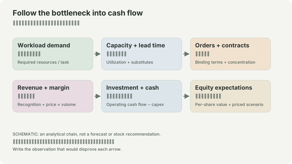
Build a conditional chain: workload change → active DRAM/HBM or persistent NAND requirement → qualified design/configuration → bit shipments and price → reported revenue. Each link can be broken by compression, model architecture, inventory, a controller change, supplier qualification, or price competition.

Exercise: map a real pipeline

Take one workload and list every object: raw data, transformed shards, checkpoint, weights, KV cache, and output. For each, record persistence requirement, approximate capacity, read/write pattern, and where it resides during one step. Run with a warm local cache, then a cold or remote source if safe. Measure data-load time separately from device execution. Finally write one DRAM hypothesis and one NAND hypothesis, each with a metric that could disprove it. The exercise produces a design question, not a ticker recommendation.